
Vadose Zone Inversion
Abstract
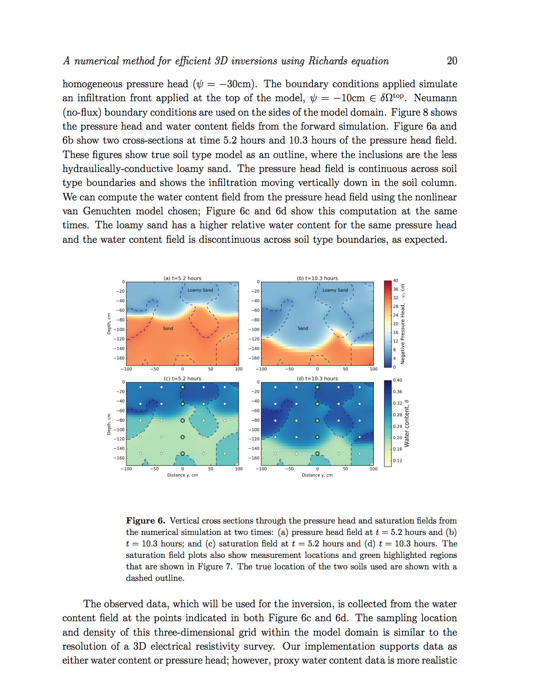
Fluid flow in the vadose zone is governed by Richards equation; it is parameterized by hydraulic conductivity, which is a nonlinear function of pressure head. Investigations in the vadose zone typically require characterizing distributed hydraulic properties. Saturation or pressure head data may include direct measurements made from boreholes. Increasingly, proxy measurements from hydrogeophysics are being used to supply more spatially and temporally dense data sets. Inferring hydraulic parameters from such datasets requires the ability to efficiently solve and deterministically optimize the nonlinear time domain Richards equation. This is particularly important as the number of parameters to be estimated in a vadose zone inversion continues to grow. In this paper, we describe an efficient technique to invert for distributed hydraulic properties in 1D, 2D, and 3D. Our algorithm does not store the Jacobian, but rather computes the product with a vector, which allows the size of the inversion problem to become much larger than methods such as finite difference or automatic differentiation; which are constrained by computation and memory, respectively. We show our algorithm in practice for a 3D inversion of saturated hydraulic conductivity using saturation data through time. The code to run our examples is open source and the algorithm presented allows this inversion process to run on modest computational resources.
Full Paper
A numerical method for efficient 3D inversions using Richards equation. On arxiv.
Highlights
Efficient algorithm for large-scale Richards equation inversions
Algorithm does not store the Jacobian, but rather computes the effect on a vector
Numerical example to recover a 3D distribution of saturated hydraulic conductivity
Open source code for forward and inverse simulation of Richards equation in 1D, 2D and 3D
Favorite Parts
If we used a finite difference algorithm to explicitly calculate each of the columns of the Jacobian with a simple forward difference, we would require a calculation for each model parameter - or approximately 8.5 years of computational time. Furthermore, we would need to recompute the Jacobian at each iteration of the optimization algorithm. In contrast, if we use the implicit sensitivity algorithm presented in this paper, we can solve the entire inverse problem in 34.5 hours.
For example, on a mesh, the explicit formation of the sensitivity requires 419 GB for five spatially distributed model parameters, which is five times the requirement for a single distributed model parameter (83.9 GB). For the implicit sensitivity on the same mesh, only 4.09 GB of memory is required, which is 1.2 times the requirement for a single distributed model parameter (3.54 GB).
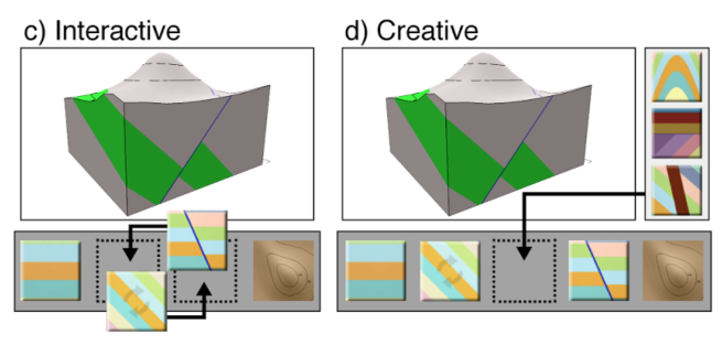
Reflecting on creating tools for technical communication.
UCalgary Geosicence - Friday Afternoon Talk Series

Podcast with Matt Hall and Graham Ganssle
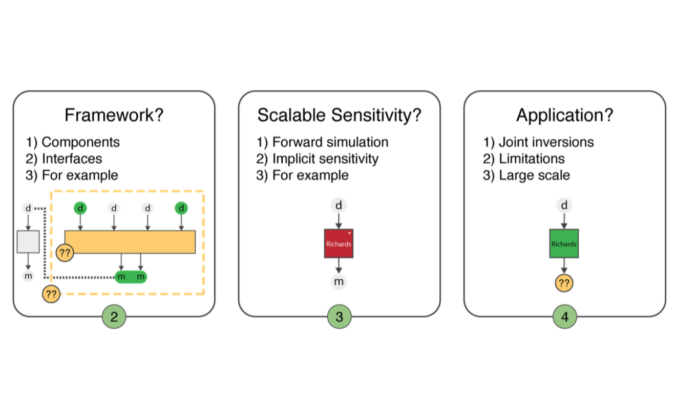
A framework for geophysical inversions with application to vadose zone parameter estimation
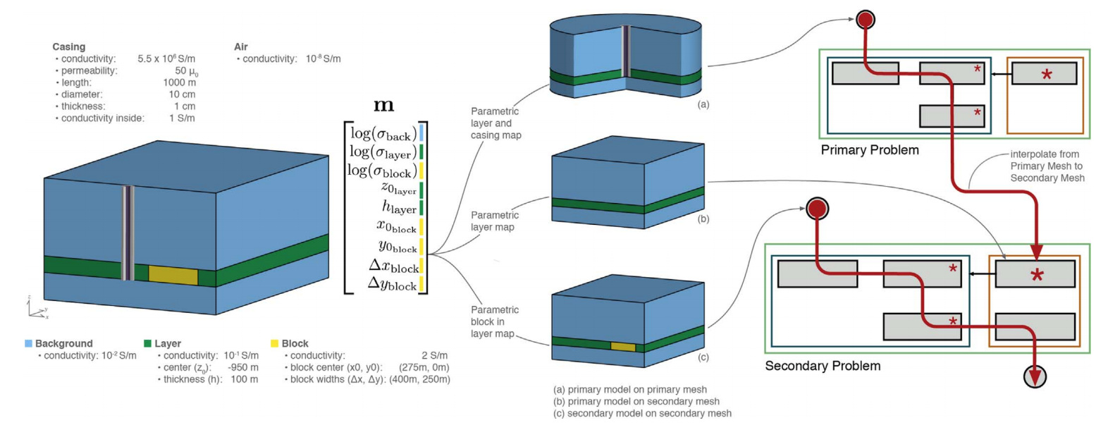
A framework for simulation and inversion in electromagnetics
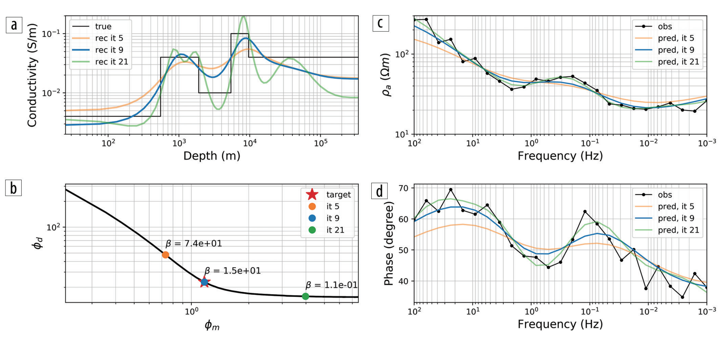
Exploring nonlinear inversions: A 1D magnetotelluric example